Akka Stream telemetry use cases
Cinnamon records essential core metrics for Akka Streams, including throughput and processing time, and extended metrics can also be enabled for recording end-to-end flow time, stream demand, latency, and per connection metrics. This guide describes and illustrates some examples and common use cases for Akka Stream telemetry.
The metric graphs in this guide have been generated from running samples with the Prometheus metric backend and Grafana for visualization.
Overall stream performance
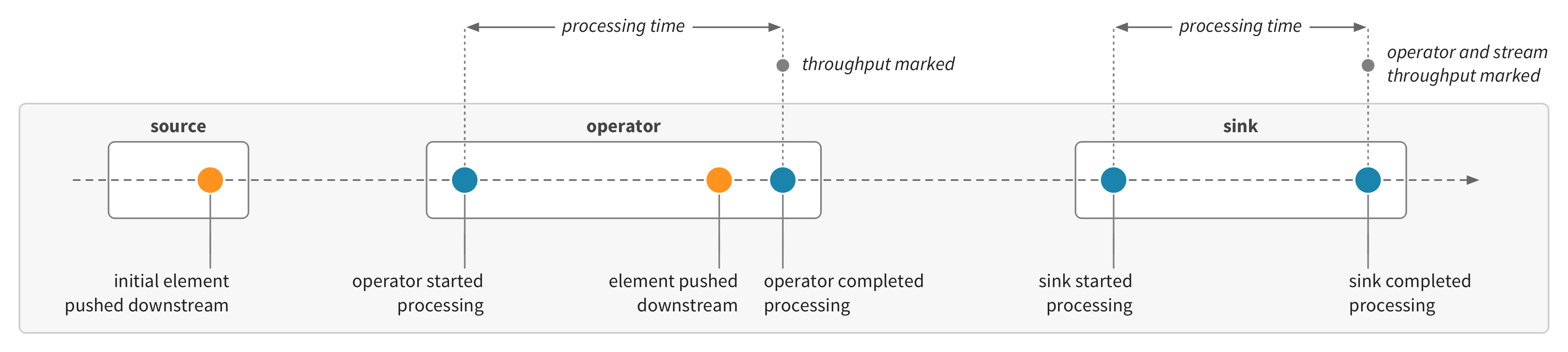
The simplest indicator for overall stream performance is the stream throughput metric, which records the rate of elements being processed through to the sinks of a stream graph. This rate is recorded as each sink completes processing:
Given this example stream:
source
.map(simulateWork(10.millis))
.map(simulateWork(20.millis))
.map(simulateWork(30.millis))
.map(simulateWork(40.millis))
.instrumentedRunWith(sink)(name = "stream-throughput")The stream throughput metric would record something like this:

Note how the throughput is related to the processing times of the operators. Akka Streams will fuse operators by default. The operators will share the same throughput, based on the combined processing time:


Slow operators
Given that the overall stream performance will be based on the slowest operators, it can be useful to visualize and compare the processing times of operators in a stream.
If we have a stream with a slow operator:
source
.map(simulateWork(10.millis))
.map(simulateWork(200.millis))
.map(simulateWork(30.millis))
.instrumentedRunWith(sink)(name = "slow-operator")Then the processing time metric will show which stage is slowest:


Also note how the throughput corresponds to the combined processing time.
The operator names include ids to uniquely identify them. These are generally ordered back-to-front, from sink to source. See stream and operator names for more information and for how to configure names.
If the sink is the slow operator, then it will show up in the same way as flow operators. Given this example stream:
source
.map(simulateWork(10.millis))
.map(simulateWork(20.millis))
.to(sink(simulateWork(300.millis)))
.instrumented(name = "slow-sink")
.run()Then the processing time metric will show the slow sink:


Akka Stream operators process flows in two directions: elements flow downstream, based on demand which flows upstream. The throughput and processing time metrics are for the processing of elements flowing downstream. Cinnamon can also record metrics for the demand flowing upstream. Demand metrics are useful for instrumenting sources, or operators which behave as sources, where the work is performed on pull in response to demand.
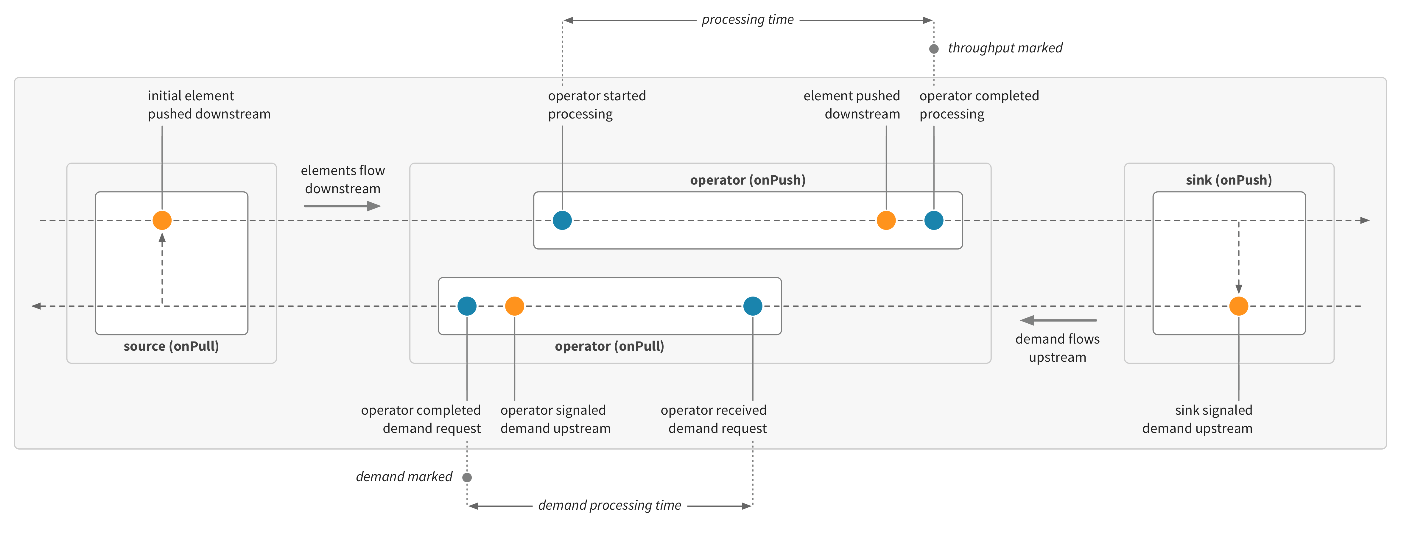
Demand metrics are not enabled by default. If demand metrics are not enabled, then Cinnamon will automatically record demand metrics for stream sources as regular metrics (so rate of demand on a source will be recorded as throughput and demand processing time for a source will be recorded as processing time).
The following example has a slow source:
source(simulateWork(300.millis))
.map(simulateWork(20.millis))
.map(simulateWork(10.millis))
.instrumentedRunWith(sink)(name = "slow-source")If demand metrics are not enabled, then the slow source will be recorded under regular processing time:


If demand metrics are enabled, then the slow source will be recorded under the demand processing time:


Some sources are actually multiple operators, in which case demand metrics will need to be enabled to measure the performance of the upstream demand flow of the subsequent operators.
Asynchronous boundaries
Akka Streams will fuse operators by default—operators will be executed within the same Actor, avoiding message passing overhead. Fused operators do not run in parallel. Asynchronous boundaries can be inserted manually, so that parts of the stream graph are processed in parallel.
If we start with a simple two-stage stream:
source
.map(simulateWork(50.millis))
.map(simulateWork(50.millis))
.instrumentedRunWith(sink)(name = "two-stage")And look at the overall performance metrics:


We can see that the overall throughput is based on the time to process elements sequentially through both operators (the combined processing time aligns with the stream throughput).
Cinnamon can record latency metrics (inactive time) for stream operators. Latency can be recorded for upstream or downstream of each operator. Latency metrics include latency (the time spent waiting for elements from upstream—the time from demanding an element upstream with a pull to starting to process an element from a push) and demand latency (the time spent waiting for demand from downstream—the time from providing an element downstream with a push to starting to process demand from a pull).
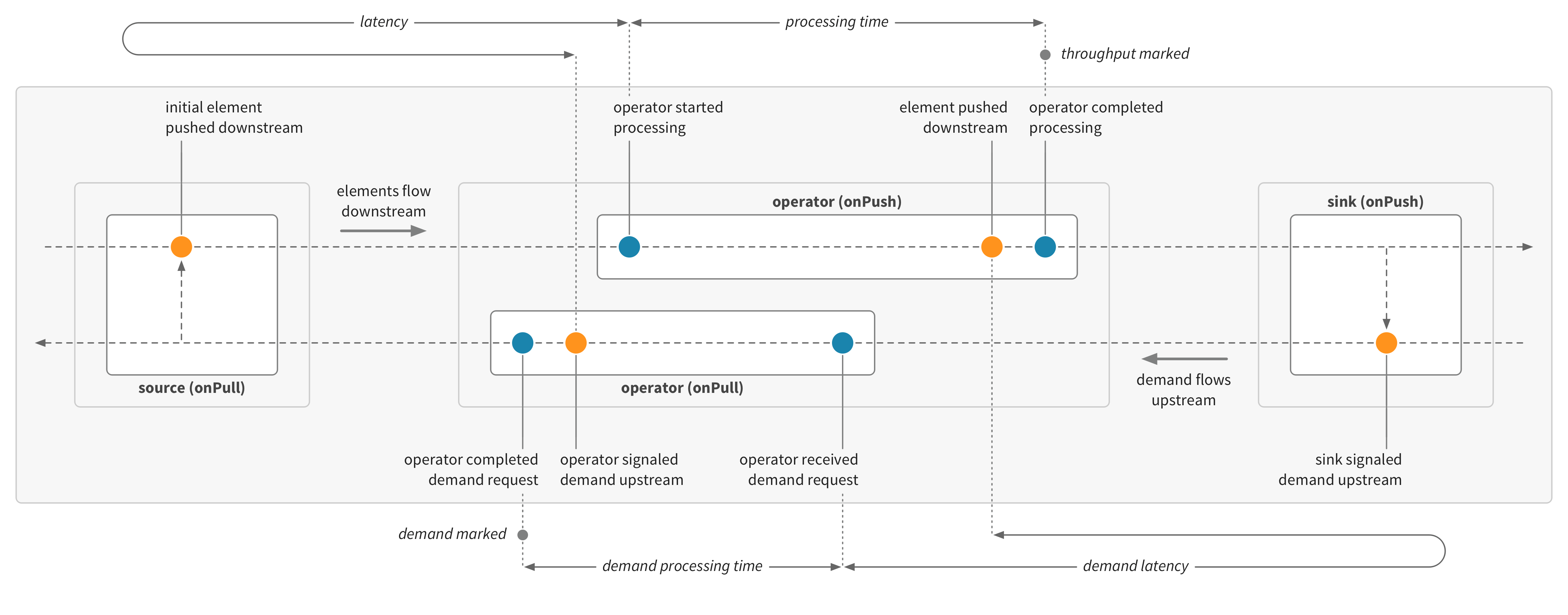
If we look at the operator latency metric for the example above, we can see that the downstream operator waits for the upstream operator to process each element first, and using the demand latency metric we can see that the upstream operator waits for the downstream operator to process each element before it receives the next demand request. The sink and source wait for both operators in the flow cycle.


Let’s add an asynchronous boundary and see how this affects performance. By adding an asynchronous boundary attribute, using the async method, each region of the stream will be executed in its own Actor—with elements passed between the asynchronous islands and buffered until there is demand from downstream.
source
.map(simulateWork(50.millis)).async
.map(simulateWork(50.millis))
.instrumentedRunWith(sink)(name = "two-stage-async")To clarify expectations, consider this analogy for the example streams above: imagine that you have a pile of dirty dishes, and there are two tasks to perform—washing each dish and drying each dish. These two tasks are the two map operations. So in the first example, with fused operations, this would be like having one person doing all the washing and drying—where they first wash a dish and then dry that dish, wash and then dry the next dish, and so on. One person is equivalent to one Actor. Fused operations is equivalent to doing all the tasks end-to-end before repeating.

If instead we had two people cleaning the dishes (two Actors), then one person could wash and the other could dry. The first person washes a dish, puts it on the dish rack (the asynchronous boundary and buffer), and can then start washing the next dish immediately. The second person takes a dish from the rack, when they’re ready, and dries the dish before putting it away. In terms of performance, we would expect that the pile of dirty dishes will be processed more quickly with two people performing the tasks in parallel. If they get into a good rhythm and the two tasks of washing and drying take around the same time, then there will often be a few dishes on the dish rack so that the second person also doesn’t need to wait. But the end-to-end flow time for dishes—the time from a dirty dish being picked up to a clean and dry dish being put away—would be longer in the version with two people, as there’s transferring the dishes (like message passing with Actors) and dishes spend some time on the dish rack (like a buffer for stream elements).
Here are the recorded metrics for the asynchronous version. The latency metrics for this version show that the two map operators, in each part of the stream, are no longer waiting for elements or demand, since the asynchronous islands are processing in parallel:


Note that the sinks and sources still wait for the operator within their asynchronous island, as expected.
The overall performance metrics show that the stream throughput for the async version is around double the stream throughput for the sequential version:


These examples use a randomly generated simulation. In this comparison, we use the same random seed so that the two streams give similar patterns and are directly comparable.
End-to-end flow metrics
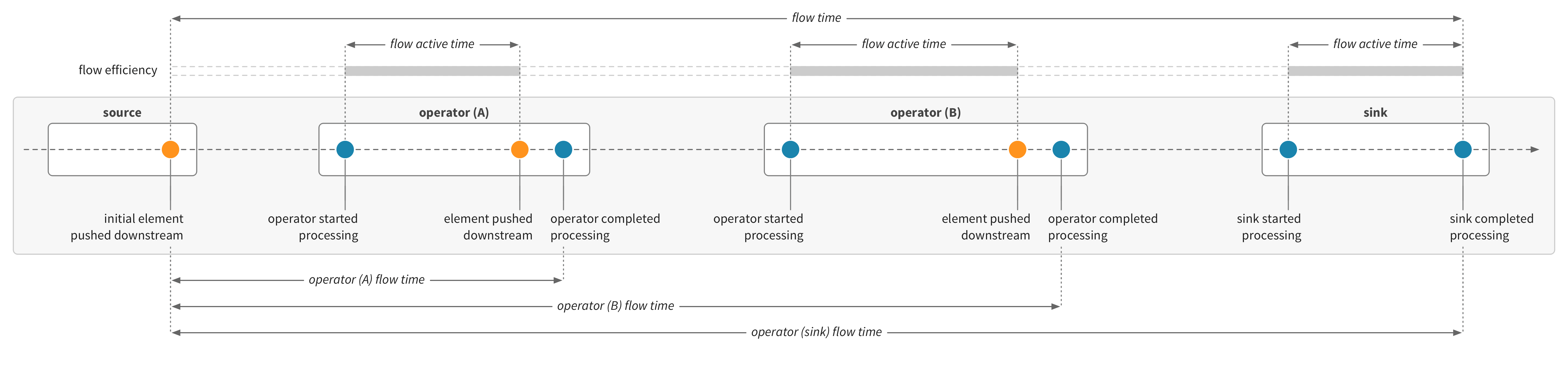
Cinnamon can have flow metrics enabled, which includes flow time—the time for elements to flow through the stream from sources to sinks. The flow time is recorded using a Stopwatch, which is started at the first push in the stream, propagated through the stream with the flow of elements, and then stopped when a sink has completed processing.
The operator flow time metric records the current flow time after each operator has completed, and can be seen as recording progress through the stream. Stopwatches can also record the active time during the flow—the time spent actively processing stream operators, as compared with waiting. A flow efficiency metric can be derived from the active time—measuring how much of the total flow time is active.
Let’s look at flow metrics for some of the simple stream examples above.
The example stream for overall stream performance is a simple linear stream with multiple operators:
source
.map(simulateWork(10.millis))
.map(simulateWork(20.millis))
.map(simulateWork(30.millis))
.map(simulateWork(40.millis))
.instrumentedRunWith(sink)(name = "flow-time", perFlow = true)The operator metrics show the expected pattern, given the simulated work times:


The overall stream throughput and the flow time will show something like this:


The flow time records the total time it takes for elements to flow through all operators, from source to sink. Because the stream operators are fused, nearly all of the flow time is active. The flow efficiency metric will be close to 100%. The operator flow time records the time so far as each operator finishes processing, and for a linear fused graph, this looks like stacking the processing times on top of each other, in flow order:


As another example, we can try the flow metrics with the examples for asynchronous boundaries above. We started with a simple two-stage stream:
source
.map(simulateWork(50.millis))
.map(simulateWork(50.millis))
.instrumentedRunWith(sink)(name = "flow-two-stage", perFlow = true)In this fused version, we get stream and flow metrics like this:


If we add the asynchronous boundary between the two parts:
source
.map(simulateWork(50.millis)).async
.map(simulateWork(50.millis))
.instrumentedRunWith(sink)(name = "flow-two-stage-async", perFlow = true)The stream and flow metrics look like this:


With the two parts processing in parallel, the overall stream throughput has doubled. The total flow time, however, is much longer than the initial fused version, while the active time is similar. This difference also gives a much lower flow efficiency. With the asynchronous boundary, each region of the stream will be executed in its own Actor—with elements passed between the asynchronous islands and buffered until there is demand from downstream. The message passing and buffering adds some amount of inactive transit time. So while the stream as a whole is processing twice as many elements, the time for elements to flow end-to-end through the stream has increased given the time to transfer elements over the asynchronous boundary.
Asynchronous operators
Asynchronous operators such as mapAsync and mapAsyncUnordered can be used to process elements concurrently—when using an API that returns Futures, or when handing off processing to an Actor (with the ask pattern). Async operators can also be used to introduce or increase parallelism, to make full use of the available resources.
In this example, we’ll start with a simple stream of two parts, but where the amount of work varies even more than in previous examples—around 10% of the time the operators will take much longer to process elements, and the downstream operator is slower than the upstream operator:
source
.via(Flow[X].map(simulateWork(0.9 -> 10.millis, 0.1 -> 100.millis)).named("one"))
.via(Flow[X].map(simulateWork(0.9 -> 40.millis, 0.1 -> 400.millis)).named("two"))
.instrumentedRunWith(sink)(name = "variable-work", perFlow = true)We’ve named the operators in this example, so that it’s easier to see which operator comes first or second. See stream and operator names for more information and for how to configure names.
The overall stream metrics give us this:


The end-to-end flow time and the throughput are aligned with each other. Because of the varying work in the simulation, we see a varying throughput.
For these examples we show time distributions, graphing both the median (0.5 quantile) and the maximum (1.0 quantile), so we can see the variation in work and time.
Looking at the processing times for the two operators, we get the expected distributions given the simulated parameters:


We can now try a version using mapAsync to parallelize the work within each operator:
source
.via(Flow[X]
.mapAsync(4)(usingFutureNamed("async-one")(simulateWork(0.9 -> 10.millis, 0.1 -> 100.millis)))
.named("one"))
.via(Flow[X]
.mapAsync(4)(usingFutureNamed("async-two")(simulateWork(0.9 -> 40.millis, 0.1 -> 400.millis)))
.named("two"))
.instrumentedRunWith(sink)(name = "variable-work-async", perFlow = true)We also use named Futures to record Scala Future metrics.
If we compare the overall stream metrics for this async version with the regular fused version, we see these results:


The throughput is higher. The flow time is also longer and we see more variation. This suggests that while the overall throughput is higher, elements also spend more time in buffers.
Here are the processing time metrics for the two mapAsync operators:


The first thing to note is that the two graphs look very similar, even though the simulated work times are different. To explore what’s happening here, let’s first check the Future metrics (which are recorded for named Futures). The completing time metric records the total time from creating a Future to it being completed with a result:


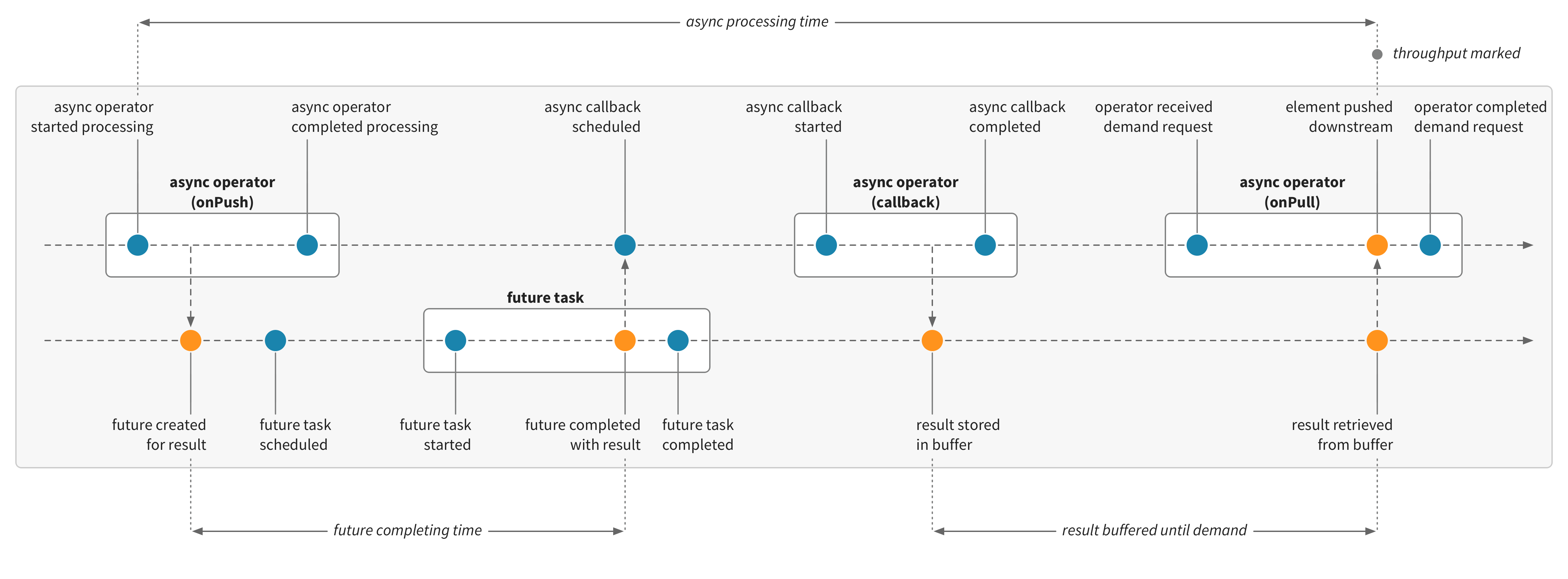
The Future metrics show the expected time distribution for the simulated work. So why are the processing times for the mapAsync operators different from the Future completing times? Asynchronous stream operators, such as mapAsync or mapAsyncUnordered, process elements by registering an asynchronous callback, which will re-enter the stream at a later time once the Future is ready, to complete the processing and pass the result downstream. This means that the regular processing time for these operators will generally be very short, with the bulk of the time spent asynchronously elsewhere, such as in a Future or Actor. To handle this, Cinnamon will detect asynchronous operators and record the processing time for these specially, using a Stopwatch. The total time for asynchronous operators will be recorded, including any asynchronous processing, and until a result is pushed downstream.
The asynchronous processing time is considered complete when elements are pushed downstream. The mapAsync operator retains the ordering of processed elements, buffering results as needed to keep the correct order. The total processing time for an element will include any time spent in buffers. The asynchronous operators will also only process elements concurrently up to the configured amount of parallelism. So in this example, the downstream operator is slower, and to retain order, the readiness of elements will be determined by the slowest Future. When the downstream operator is at parallel capacity, it will not signal demand to the upstream operator, which then also effectively waits for the slowest task. So we can see that the overall behavior is constrained by the slowest processing stage.
As shown in the example for asynchronous boundaries, we can record latency metrics (inactive time) for stream operators. Here is the demand latency for the first operator (the time spent waiting for demand from downstream) and the latency for the second operator (the time spent waiting for elements from upstream):


We can see how the time distribution for the upstream operator when waiting for demand from the downstream operator reflects the downstream processing time.
If we don’t require the order of elements to be preserved, then we can use mapAsyncUnordered to increase throughput. While mapAsync will retain ordering—only emitting elements when preceding Future results have been pushed downstream—mapAsyncUnordered will emit elements as soon as results are available. Here’s the same example using mapAsyncUnordered:
source
.via(Flow[X]
.mapAsyncUnordered(4)(usingFutureNamed("async-unordered-one")(simulateWork(0.9 -> 10.millis, 0.1 -> 100.millis)))
.named("one"))
.via(Flow[X]
.mapAsyncUnordered(4)(usingFutureNamed("async-unordered-two")(simulateWork(0.9 -> 40.millis, 0.1 -> 400.millis)))
.named("two"))
.instrumentedRunWith(sink)(name = "variable-work-async-unordered", perFlow = true)We can see the increased overall stream throughput:


The end-to-end flow time is also shorter than the mapAsync version, and closer to the version using fused operators.
The processing time metrics for the two operators give this pattern:


The Future completing time metrics for the underlying tasks are identical to those for the mapAsync version above, as expected:


As in the mapAsync version, the latency metrics for the mapAsyncUnordered version show the way that the upstream operator is backpressured by the slower downstream operator (but not to the same degree):


Tracing streams
Cinnamon has OpenTracing integration for Akka Streams. While metrics provide an aggregated view over time of a stream’s behavior, traces record specific dataflows or execution paths through a stream or distributed system. The tracing integration builds on underlying context propagation instrumented by Cinnamon, which is also used for the end-to-end flow metrics or recording processing time for asynchronous operators).
We can look at traces for some of the simple stream examples above.
If we enable tracing for the example stream from overall stream performance:
source
.map(simulateWork(10.millis))
.map(simulateWork(20.millis))
.map(simulateWork(30.millis))
.map(simulateWork(40.millis))
.instrumentedRunWith(sink)(name = "traced", traceable = true)Then traces will be recorded and can be reported to tracing solutions, such as Zipkin:

Here’s the example stream using mapAsync from asynchronous operators, enabled for tracing:
source
.via(Flow[X]
.mapAsync(4)(usingFutureNamed("async-one")(simulateWork(0.9 -> 10.millis, 0.1 -> 100.millis)))
.named("one"))
.via(Flow[X]
.mapAsync(4)(usingFutureNamed("async-two")(simulateWork(0.9 -> 40.millis, 0.1 -> 400.millis)))
.named("two"))
.instrumentedRunWith(sink)(name = "traced-async", traceable = true)A trace reported to Jaeger looks like this:

In this trace, the full asynchronous processing time for the async operators is recorded. As for the operator processing time metric, Cinnamon will complete the trace span for async operators when they push elements downstream. The trace also includes trace spans for the named Futures. Cinnamon tracing and context propagation works across supported instrumentations, so a trace will continue through streams, actors, futures, and HTTP requests.